TUFLOW FV MATLAB Toolbox
| USEFUL LINKS | ||
| Wiki Links | Help | Downloads |
| TUFLOW FV Wiki Main Page | Products Support/Contact | TUFLOW FV Downloads |
| TUFLOW FV Tutorials | Requesting a Licence | Tutorial Module Data |
| TUFLOW Classic/HPC Wiki | TUFLOW FV Glossary | Manuals |
Introduction
The purpose of this page is to help get you setup with the TUFLOW FV MATLAB Toolbox and to provide examples that demonstrate its use. (tfv).
The TUFLOW FV MATLAB Toolbox is a suite of tools for post-processing results from the TUFLOW FV hydrodynamic, sediment transport, water quality and particle tracking modelling software.
The MATLAB examples presented herein use Tutorial Module 5 as the example dataset.
Toolbox Overview
MATLAB
These tools require MATLAB installed. The tools have been designed to allow new users to be able to quickly and easily visualise model output. If you're more experienced with MATLAB it also offers an easy platform to build customised visualisations from. Please note these tools have been developed using MATLAB version R2022a. For versions older than R2022a please use some caution as there may be incompatibilities with the toolbox.
The documentation on this page assumes you are familiar with MATLAB and MATLAB graphics objects.
FVG Suite
The accompanying tools rely on object oriented programming to provide a simple front-end interface that is similar to MATLAB built-in components. The tools are based on an fvgraphics object that creates a figure with a scrollbar inside it. The fvgraphics object stores the information necessary to scroll through timesteps and tell other objects to update the images. FVG objects can then be placed in any axis that is created within the fvgraphics object. FVG objects include patch objects that represent mesh cells and are coloured based on the model results. The FVG objects call their own respective FV-Res objects which are responsible for extracting the results from the TUFLOW FV results file and then sending a signal back to the FVG object to update the patches.
Download And Setup
Download Toolbox
To download the TUFLOW FV Matlab Toolbox please visit the TUFLOW Website.
Within the download package are the following folders:
| File or Directory | Description |
|---|---|
| .\log\ | Pre-run log file outputs used for the example scripts. |
| .\results\ | Pre-run NetCDF outputs used for the example scripts. |
| .\toolbox\ | Pre-run NetCDF outputs used for the example scripts. |
| .\tutorial\ | Series of example scripts. |
Unzip and save the download package to a preferred location on your local drive or network. For this example the package has been saved to C:\MATLAB\TUFLOWFV_MATLAB_Toolbox.
Adding Toolbox
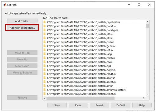
- To get the required tools setup firstly add the TUFLOW FV MATLAB Toolbox to your MATLAB path. Depending on your version of MATLAB the set path button will be similar to this:
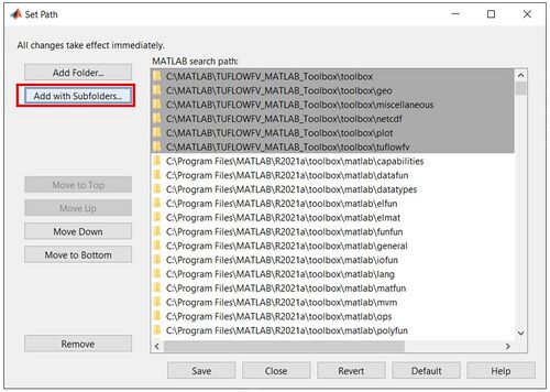
- Then add with subfolders:
- And select the toolbox folder from your save location. For example: C:\MATLAB\TUFLOWFV_MATLAB_Toolbox\toolbox.


You have now setup your MATLAB environment. Next we will use the provided tutorial scripts to test out the TUFLOW FV MATLAB Toolbox.
Visualising Tutorial Module 5 Results
Tutorial Module 5 demonstrates the development of a 3D estuary model. Starting with a 2D model, the tutorial progressively increases in complexity, incorporating layers and density coupling to observe stratification in an estuary. Before completing the following exercises, if you have not already done so please download the data package for the tutorial from the TUFLOW FV Tutorial / Demo Models page located at www.tuflow.com.
MATLAB Profile
To view the results of the HYD_000 and HYD_001 simulations we will produce profile plots for salinity. A profile plot will allow you to view a variable through the vertical as a timeseries (with time slider bar).
Writing A Profile NetCDF File
In order to produce timeseries and profile plots, a profile NetCDF (nc) file must be written using the output NetCDF file from TUFLOW FV. To write a profile file, please navigate to \tutorial\visual\1.timeseries\ and open the script ‘ts_000_create_profile_file.m’ in MATLAB. Verify that the following lines of code are set to process data from the HYD_000, HYD_001 and HYD_002 models.

This script will generate NetCDF profile files with the simulation results located at the 9 output sites specified on lines 21 to 29 as shown below:

Run the script. The associated model profile files (‘HYD_000_PROFILES.nc’, ‘HYD_001_PROFILES.nc’ ... etc.) will now be generated in the results folder.
If you are currently completing Tutorial Module 5 you can return to create a timeseries plot.
Profile Plot
Once profile files have been written, profile plots can be produced. To produce profile plots, navigate to \tutorial\visual\2.profiles\ and open the script ‘pf_000_plot_profiles’. This script will create a vertical profile of elevation vs. a 3D variable from a profile file. Make the appropriate changes shown below to plot salinity at point 1 for the HYD_001 model.

An example of a profile plot for HYD_001 is shown below:
HYD_001: 3D model

If you are currently completing Tutorial Module 5 you can return to the 3D profile results discussion.
MATLAB Timeseries
A timeseries plot allows you to view the changes to a variable over time. This can be useful for determining when a model converges to a solution from initial values. To view the results of the HYD_000 temperature simulation we will produce a timeseries plot for temperature. In order to produce timeseries and profile plots, a profile NetCDF (nc) file must be written (please refer to Writing a profile NetCDF file).
Timeseries Plot
A timeseries plot allows you to view the time series of a single variable at a single location. To produce a timeseries plot, please go to \tutorial\visual\1.timeseries\ and open the script ‘ts_001_plot_2D_variable_timeseries.m’ in MATLAB. Change lines 16, 17, 18 and 28 to produce a plot for temperature at point 4. The final code after these changes have been made is shown below.

If you run the script at point 4, you should see a plot similar to the one shown below:

If you are currently completing Tutorial Module 5 you can return to the timeseries results discussion.
MATLAB Sheet
To produce a sheet plot, please navigate to \tutorial\visual\3.sheets and open the script 'sh_000_plot_sheet.m'. As an example for how to configure the script please complete the following steps to produce a temperature sheet for the HYD_000 model.
- Point the script to the TUFLOW FV results file (TFV_resfile) for HYD_000, '../../../results/HYD_000.nc',
- Change the variable (var) to 'TEMP',
- Change the colour limits (clim) to [10 20],
- Change the title name (long_name) to 'Temperature (deg C)'.

Run the script and use the time slider bar to observe how the temperature gradient is developed in the estuary:

Sheet Plot with Vectors
As identified in the timeseries plots, oscillation in temperature is observed, presumably due to the tide. To further investigate how the temperature is affected by the tide and boundary conditions, a sheet plot of temperature with velocity vectors can be produced.
To produce a sheet plot with vectors, please navigate to \tutorial\visual\3.sheets and open the script 'sh_000_plot_sheet_with_vectors.m'. Please follow the steps below to produce a temperature sheet plot with velocity vectors.
- Point the script to the TUFLOW FV results file (TFV_resfile) for HYD_000, '../../../results/HYD_000.nc',
- Change the sheet variable (sheet_var) to 'TEMP',
- Ensure the vector variable (vec_var) is set to 'V',
- Change the colour limits (clim) to [10 20],
- Change the title name (long_name) to 'Temperature (deg C)'.

Run the script and use the time slider bar to observe how temperature is affected by the tide in the estuary.
Some sheet plots with vectors produced in MATLAB are shown below:

If you are currently completing Tutorial Module 5 you can return to the Initial 2D model HYD_000.
MATLAB Curtain
To view the results with density coupling we will produce a curtain plot. A curtain plot allows you to view a variable along a cross section as a function of chainage and depth (with time slider bar). The curtain plot will allow us to see the formation of a salt wedge in the estuary.
Curtain Plot
To produce a curtain plot, please navigate to \tutorial\visual\4.curtains\ and open the script ‘cu_000_plot_curtain.m’. This script will create a cross sectional profile for a 3D variable using both the model results file and model geofile as inputs. The cross section to be plotted is along the polyline specified on lines 22 to 49 as shown below:

Make the appropriate changes shown below to plot a curtain for salinity for the HYD_002 model.

Run the script for HYD_002. Slide the time control bar across to the final point, at 00:00 on the 7th of May. You should see the following plot:

If you are currently completing Tutorial Module 5 you can return to the 3D model with density coupling HYD_002.
FVG Visualisation Tutorials
The following tutorials show further basic uses of the FVG visualisation suite. For more advanced uses, and questions on usage, please email support@tuflow.com.
Conclusion
Thanks for working through the TUFLOW FV MATLAB Toolbox tutorial page. We hope it has been useful. If you have any questions or would like to contribute please get in contact with us via support@tuflow.com. Please return the TUFLOW FV Wiki Main Page and happy modelling.