TUFLOW FV Python Toolbox Archive
Please note this page has been superseeded by the new TUFLOW FV Python Toolbox page.
| USEFUL LINKS | ||
| Wiki Links | Help | Downloads |
| TUFLOW FV Wiki Main Page | Products Support/Contact | TUFLOW FV Downloads |
| TUFLOW FV Tutorials | Requesting a Licence | Tutorial Module Data |
| TUFLOW Classic/HPC Wiki | TUFLOW FV Glossary | Manuals |
Introduction
The purpose of this page is to help get you setup with Python and to provide examples that demonstrate use of the TUFLOW FV Python Toolbox (tfv).
The tfv package is a suite of tools for post-processing results from the TUFLOW FV hydrodynamic, sediment transport, water quality and particle tracking modelling software.
The help page can be broken up into the following sub-sections:
Install Python
There are a range of options for installing Python on your computer. You can either download through a package (such as Anaconda) or directly download from the Python Website. For this example we will install the basic Python installation and then install further modules using pip.
To install Python please visit the Python Download Page and download the most recent executable download file for windows. Run the installation by following these steps:
Install Python Integrated Development Environment
Once you have downloaded and installed Python, the next step is to download a Python Integrated Development Environment (IDE) to edit, run and debug your code. Whist there are a range of different IDEs out there this example will use the IDE PyCharm. We have chosen PyCharm because it has some nice tools for handling virtual environments which will help keep us organised later if we need to work with different Python libraries and versions.
Proceed to download PyCharm using the most recent executable download file for windows and run the installation. PyCharm Community and Educational are open-source projects.
Setup Python Environment
Following successful installation of Python and Pycharm we will setup a virtual environment within Pycharm and install the TUFLOW FV Python Toolbox including its package dependencies. Please work through each of the steps as follows:
- Open PyCharm and create a new project.
- Set the project location and a create virtual environment. Click OK.
- Goto: File >> Settings and open up the project interpreter options.
- Click the plus button to select new modules for installation.
- Select the tfv package and click install package (Noting there may be a more recent version than 0.0.8).
- The installation should complete successfully and install the required dependencies for tfv.
You have now successfully setup your Python Environment.
If you're not using PyCharm the tfv package is available via the Python Package Index PyPi. You can optionally select to install it via the command prompt or terminal using pip as follows:
python -m pip install tfv
Next we will download the example tutorial script files and include them in our project.
Download Example Datasets and Scripts
Please download the archive example scripts used in this tutorial from the https://downloads.tuflow.com/Utilities/TUFLOW_FV_Python_Toolbox/TUFLOW_FV_Python_Toolbox_Archive.zip
Within the download package are the following folders:
| File or Directory | Description |
|---|---|
| .\tutorial\basic | Simple example plots using the tfv TUFLOW FV Python Toolbox. |
| .\tutorial\extended | More advanced plots that build on the basic examples. |
| .\results | Some pre-cooked results from Tutorial Module 5 if you don't have time to work through the full tutorial. |
| .\Readme_and_Install_Notes.txt | Short description of each script and basic metadata. |
Plot Example 1: Timeseries
A timeseries plot allows you to view the timeseries data of a single variable at a single location. In order to produce timeseries plots, a profile NetCDF (nc) file must be written using the results NetCDF file from TUFLOW FV.
Profile File
To write a profile file, please open the script tutorial\basic\000_create_time_series_file.py in PyCharm (or your preferred IDE). Verify that the following lines of code are set to process data from the HYD_000, HYD_001 and HYD_002 models.

This script will generate NetCDF profile files with the simulation results located at the 9 output sites specified above.
Run the script. The files ‘HYD_000_time_series.nc’, ‘HYD_001_time_series.nc’ and ‘HYD_002_time_series.nc’ will now be generated in the output folder. If prompted by overwrite warnings simply type 'y' to recreate the time series files. They are not large and shouldn't take long to reprocess.
Timeseries
To plot the previously created profile file, open tutorial\basic\001_plot_2D_variable_timeseries.py. This script will create a timeseries plot of elevation vs. a variable selected from a profile file. Make the appropriate changes shown below to plot temperature at point 4 for HYD_001.

As shown above, the path to the results and profile files must be provided. Additionally, depending on which point you would like to plot a profile for, you will have to enter the point name and coordinates as provided in the comment lines. Finally, depending on which variable you wish to plot, you may have to alter the var, y_lim, and y_label lines of code.
A timeseries plot produced in python is shown below:
Plot Example 2: 3D Profile
To view the results of the HYD_001 3D simulation (no density coupling) we will produce a profile plot of salinity.
Open tutorial\basic\002_plot_profile.py. This script will plot elevation vs. salinity at a given timestep and point location allowing you to review the vertical variation of the variable. You can then move forward or backward in time via the timeslider. Make the appropriate changes shown below to plot salinity at point 1 for HYD_001 and run the script.

As shown above, the path to both the results directory and the name of the results file must be provided. Additionally, depending on which point you would like to plot a profile for, you will have to enter the coordinates as provided in the comment lines. Finally, depending on which variable you wish to plot, you may have to alter the var, x_limit, and x_label lines of code.
An example of a profile plot produced in python is shown below:

Plot Example 3: Sheet
To produce a sheet plot with vectors open tutorial\Basic\003_plot_sheet.py. This script will visualise a given variable in plan view. Make the appropriate changes shown below to plot the temperature distribution for the HYD_000 model.

As shown above, the path to the results file must be provided. Additionally, depending on which variable you wish to plot, you may have to alter the var, var_name, and var_lim lines of code.
A sheet plot for temperature with vectors produced in Python is shown below:

If you are currently completing Tutorial Module 5 you can return to the sheet plot discussion. For others please continue to further examples.
Plot Example 4: Curtain
A curtain plot allows you to view a variable along a cross section as a function of chainage and depth.
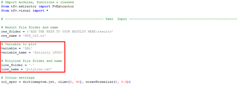
Open tutorial\basic\004_plot_curtain.py. The cross section will be plotted along the polyline as specified in the code (see below). Make the appropriate changes shown below to plot the salinity distribution for the HYD_002 model.
A curtain plot for salinity produced in Python is shown below:
Plot Example 5: Combined
To create this plot you will need to ensure that you've created a profile timeseries as a prerequisite. If you have have your time_series.nc outputs already then please open tutorial\Extended\5.combined_plots\co_000_plot_multiple_ways.py.
This script will plot a profile, timeseries, sheet and curtain plot of velocity on a single figure.
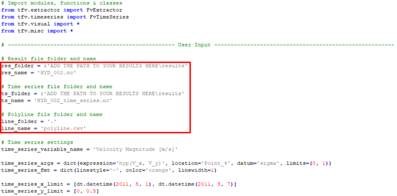
In the user input section of the code please ensure that the paths to both the results and profile files are provided. Then proceed to change the code accordingly for your chosen profile/timeseries as well as sheet and curtain variables. As an example, make the appropriate changes shown below to produce all four plots for velocity, including profile and timeseries plots at point 3, for the HYD_002 model.

As shown above, depending on which point you would like to plot a profile for you will need to enter the point name and coordinates as provided in the comment lines.
A combined plot for velocity produced in Python is shown below:
Conclusion
Thanks for taking a look at the TUFLOW FV Python Toolbox. We hope this page was useful. If you have any ideas for new additions to the page please let us know via support@tuflow.com. Please return the TUFLOW FV Wiki Main Page and happy modelling.


